📰 Trending Topics
Google News - Trending
Google News - Technology
Apple to lease iPhones, other products to users through Klarna partnership - Fox Business
2026-07-28 17:58
- Apple to lease iPhones, other products to users through Klarna partnership Fox Business
- Apple will now let you lease your next iPhone or Mac instead of buying it CNN
- Apple Upgrade Is A Great Deal On Paper, But Make Sure You Read The Fine Print Engadget
- Apple Upgrade launches in the United States Apple
- You Can Lease a New iPhone, iPad, or Mac Starting at $12 a Month PetaPixel
Galaxy Z Fold 8’s wide new design is reportedly selling faster than Samsung expected - 9to5Google
2026-07-28 16:21
- Galaxy Z Fold 8’s wide new design is reportedly selling faster than Samsung expected 9to5Google
- Samsung’s Galaxy Z Fold 8 ‘Passport’ Design Is the Next Big Smartphone Trend Bloomberg.com
- Samsung Galaxy Z Fold8 Ultra, Fold8 and Flip8: Foldables, Perfected for Every Way of Living Samsung Global Newsroom
- Score a free Samsung Galaxy Z Fold 8 with AT&T’s latest deal Mashable
- How to Get Samsung’s Galaxy Z Fold 8 for $599 Droid Life
Claude chats exposed in Google searches – another endorsement of Apple’s privacy approach - 9to5Mac
2026-07-28 12:16
- Claude chats exposed in Google searches – another endorsement of Apple’s privacy approach 9to5Mac
- Some people's chats with Claude AI found to be publicly available online BBC
- Private Claude Conversations Have Been Indexed by Search Engines CNET
- Your public Claude app may be searchable on Google Axios
- PSA: Your Claude shared chats and Artifacts may have ended up on Google TechCrunch
Granola launches an Apple Watch app - TechCrunch
2026-07-28 13:00
- Granola launches an Apple Watch app TechCrunch
- Apple Watch just gained a brand-new app for AI meeting notes 9to5Mac
- Granola Apple Watch App Explained: Features, Privacy Gaps, and Timing Gadget Hacks
- Granola AI Meeting Notes App Launches Handy Apple Watch Version The Mac Observer
- Granola launches Apple Watch app to record and transcribe meetings Межа. Новини України.
NASA - Breaking News
Smoke Blankets Oregon
2026-07-28 04:01

Dry thunderstorms that popped up over the Cascade Range on the evening of July 15, 2026, peppered Oregon and Washington with thousands of lightning strikes as they moved east across the states. By the following day, NASA satellites had begun to detect large numbers of wildland fires burning throughout central and eastern Oregon.
Though initially small, these blazes strengthened as they were fanned by gusty winds and raced through landscapes parched by extreme drought and baking in summer heat. When NASA’s Aqua satellite captured the image shown above on the afternoon of July 26, smoke poured northeast from dozens of large fires that had collectively charred hundreds of square miles. The fires produced a blanket of haze, prompting state officials to issue air quality advisories for eastern Oregon.
Many communities faced evacuation orders as more than 10,000 firefighters battled wildfires throughout the state. On the day the image was captured, the largest active fires were the Hay Creek Complex, Brewer, Big Grass, Akawa Butte, and Powder River fires. Several of these blazes were less than 5 percent contained, according to the National Interagency Fire Center. State officials invoked Oregon’s Emergency Conflagration Act to protect communities as they responded to particularly threatening fires such as the Shingle, Bench, Beachcomb, and Second Flat fires.
Government satellite data are part of a global system of observations used to track fire behavior and analyze emerging trends. Among the real-time wildfire monitoring tools that NASA makes available are FIRMS (Fire Information for Resource Management System), the Worldview browser, and the Fire Event Explorer.
As of July 27, 2026, fires in Oregon had burned more than one million acres, according to news outlets. Meanwhile, the National Interagency Fire Center reported that fires had burned more than 4 million acres across the United States. The 10-year average (2016-2025) for this point in the season is 3.4 million acres.
NASA Earth Observatory image by Michala Garrison, using MODIS data from NASA EOSDIS LANCE and GIBS/Worldview. Story by Adam Voiland.

References & Resources
- Central Oregon Fire Info (2026, July 27) The Source For Comprehensive Fire, Health, And Air Quality Information In Central Oregon. Accessed July 27, 2026.
- KGW8 (2026, July 27) Latest updates on Oregon wildfires: Fires burn more than 1 million acres across the state. Accessed July 27, 2026.
- NASA Earthdata (2026) Wildfires. Accessed July 27, 2026.
- National Interagency Fire Center (2026) Oregon. Accessed July 27, 2026.
- Northwest Interagency Coordination Center (2026, July 27) Official Fire Information. Accessed July 27, 2026.
- OPB (2026, July 27) Oregon wildfires explode over weekend with no signs of slowing down. Accessed July 27, 2026.
- Oregon State Fire Marshal (2026, July 27) OSFM Wildfire Info. Accessed July 27, 2026.
- Oregon.gov (2026, July 26) Current wildfire info. Accessed July 27, 2026.
- Oregon Smoke Information (2026, July 27) Air quality advisory for Eastern Oregon and parts of Central Oregon. Accessed July 27, 2026.
- Oregon Department of Forestry (2026, July 27) Latest News. Accessed July 27, 2026.
- U.S. Drought Monitor (2026, July 21) Oregon. Accessed July 27, 2026.
You may also be interested in:
Stay up-to-date with the latest content from NASA as we explore the universe and discover more about our home planet.
Dry, warm, and windy conditions across the U.S. Great Plains led to extreme fire activity in March 2026.
The blaze burned more than 150 square miles and swept through parts of a ski resort.

Firefighters are battling two destructive blazes in the southern part of the state as drought grips the U.S. Southeast.


NASA Astronaut Chris Williams to Discuss Space Station Mission
2026-07-27 18:49

NASA astronaut Chris Williams will recap his recent eight-month mission aboard the International Space Station during a news conference at 2:45 p.m. EDT Tuesday, Aug. 4, from the agency’s Johnson Space Center in Houston.
NASA will stream this event live through a variety of platforms. Learn where to watch online:
United States-based media interested in attending in person must contact the NASA Johnson newsroom no later than 5 p.m., Friday, July 31, at jsccommu@mail.nasa.gov.
Media wishing to participate by phone must contact the Johnson newsroom no later than two hours before the start of the event. To ask a question by phone, media must dial into the news conference no later than 15 minutes prior to the start of the call. NASA’s media accreditation policy is available online.
Williams returned to Earth on July 26, after logging 241 days as an Expedition 73/74 flight engineer during his first spaceflight. He returned along with Roscosmos cosmonauts Sergey Kud-Sverchkov and Sergei Mikaev, completing 3,856 orbits of the Earth over the course of their more than 102-million-mile journey. They also saw the arrival of six visiting spacecraft and the departure of eight.
During his mission, Williams supported a wide range of scientific investigations and technology demonstrations. He helped advance research for new cancer treatments and improved in-space manufacturing of materials used in high-performance computers and electronics. Williams also completed two spacewalks to prep for space station power system upgrades and to replace a faulty joint on the Canadarm2 robotic arm. The crew’s work aboard the space station helps improve life on Earth and prepare for future human missions to the Moon and Mars.
To learn more about International Space Station research, operations, and its crews, visit:
-end-
Joshua Finch
Headquarters, Washington
202-358-1100
joshua.a.finch@nasa.gov
Anna Schneider
Johnson Space Center, Houston
281-483-5111
anna.c.schneider@nasa.gov
NASA Science Soars During August Total Solar Eclipse
2026-07-27 18:01
6 min read
NASA Science Soars During August Total Solar Eclipse
Each time the Moon covers the Sun during a total solar eclipse — darkening daytime skies and briefly revealing the Sun’s ethereal outer atmosphere, the corona — it presents new opportunities to better understand our star and its influence on Earth.
On Wednesday, Aug. 12, as the next total solar eclipse sweeps over Greenland, Iceland, and Spain, NASA-funded science teams will be chasing the Moon’s shadow with a high-altitude jet and scientific balloons to investigate the Sun’s dynamics and how the temporary darkening of our skies affects our atmosphere.
“From our unique perspective on Earth during a total solar eclipse, scientists can study the Sun’s corona in a way we can’t from anywhere else in the solar system,” said Kelly Korreck, eclipse program manager at NASA Headquarters in Washington. “The Sun impacts our daily life, satellites, and astronauts in space, and we can take advantage of this moment to advance our understanding of that influence.”
High-flying jet to record solar dynamics
Soaring in the nose cone of NASA’s WB-57 high-altitude research aircraft is a suite of four cameras to take high-resolution images of the corona in several different wavelengths of visible and infrared light. Part of an instrument developed by the NASA Scientifically Calibrated In-Flight Imagery (SCIFLI) team at NASA’s Langley Research Center in Hampton, Virginia, the cameras will capture at least 20 images per second, recording structures, outflows, and rapid changes in the corona during the total solar eclipse.
With these images, scientists hope to learn more about the formation of prominences (solar material that gets suspended above the Sun’s surface), better understand the corona and how it gets heated to nearly a million degrees, and investigate how material in the corona and the solar wind are related, which flows out from the Sun across the solar system.

By chasing the Moon’s shadow, the jet will extend how long the cameras can observe the corona. On the ground, the longest anyone will be able to see the corona is two minutes and 18 seconds. But flying along the eclipse path at 460 miles per hour, the jet’s view of the corona will last nearly three minutes.
NASA’s WB-57 will fly at 50,000 feet, above any clouds that might obscure the view of the corona from the ground. The altitude also allows the cameras to observe some infrared wavelengths that get absorbed by the lower atmosphere before reaching the ground, and the corona only has been observed in those wavelengths a few times before.

The instrument, called SCIFLI Multispectral Airborne Imager, or SAMI, also flew on a WB-57 during the total solar eclipse on April 8, 2024, providing valuable imagery and information about the corona. However, the study’s principal investigator, Amir Caspi of the Southwest Research Institute in Boulder, Colorado, says each total solar eclipse provides new opportunities to learn more about the corona.
“The Sun is always changing,” Caspi said. “Every eclipse is different. So we could see things we didn’t see before. And we learn from each eclipse how to better observe the next one.”
Caspi’s team also is making some enhancements for the 2026 campaign based on lessons learned in 2024. For example, the team will adjust exposure times to better capture bright features that were overexposed in 2024 imagery. They will also leverage software developed since 2024 to process and analyze the data sooner than before.
The experiment is funded by NASA’s Heliophysics Low Cost Access to Space Program.
Balloons to watch atmospheric changes
When a total solar eclipse suddenly turns daytime skies dark, our atmosphere changes in ways we don’t yet fully understand.
The NASA-supported Nationwide Eclipse Ballooning Project, led by Angela Des Jardins at Montana State University, is sending students from several U.S. universities to Iceland and Spain to launch scientific balloons before, during, and after the eclipse to better understand those changes.

In Iceland, two teams will launch a total of 80 balloons starting 18 hours before the eclipse until eight hours afterward to study how the eclipse affects Earth’s “boundary layer,” the part of the atmosphere that touches the ground. The thickness of the boundary layer changes depending on factors such as surface temperature and moisture in the air.
Previous balloon flights during solar eclipses in October 2023 and April 2024 showed that the boundary layer collapsed, or decreased in thickness, in locations with clear skies but not where there were cloudy skies. Scientists wonder whether that will be different in Iceland in 2026. Changes in the boundary layer are driven by the day-night cycle. However, in Iceland in August, the days are long and nights are short, so the nighttime influences might not be as strong as in 2023 or 2024.
“Will this eclipse be able to collapse the boundary layer?” said Matthew Bernards, a chemical engineering professor at the University of Idaho, who leads one of the Iceland teams.
In Spain, three balloon teams will launch a total of six balloons with 360-degree cameras to image the eclipse shadow from above. These balloons also will include instruments designed to measure levels of ozone in the atmosphere, which requires sunlight to form. Similar balloon experiments showed that ozone decreased during totality in April 2024. Scientists wonder whether there will be differences with this eclipse, particularly since it happens at a later time of day and during a different season.
Follow along
While the total solar eclipse won’t be visible in the U.S., some parts of the country will be able to see a partial solar eclipse. Learn more about where to see the eclipse and how to view it safely.
by Vanessa Thomas
NASA’s Goddard Space Flight Center, Greenbelt, Md.
Lee esta historia en español aquí.
Share
Details
Related Terms
Explore More


NASA Astronaut Chris Williams Returns to Earth
2026-07-27 16:48

NASA astronaut Chris Williams is all smiles in this July 26, 2026, photo taken shortly after he landed with Expedition 74 Roscosmos cosmonauts Sergey Kud-Sverchkov, and Sergei Mikaev in Kazakhstan. This was Williams’ first mission.
Williams spent eight months aboard the International Space Station, where he supported a wide range of scientific investigations and technology demonstrations. He also completed two spacewalks to prep for space station power system upgrades and to replace a faulty joint on the Canadarm2 robotic arm.
Image credit: NASA/Bill Ingalls
NASA’s Swift Sees ‘Wandering’ Mega Black Hole Shredding Star
2026-07-27 16:06
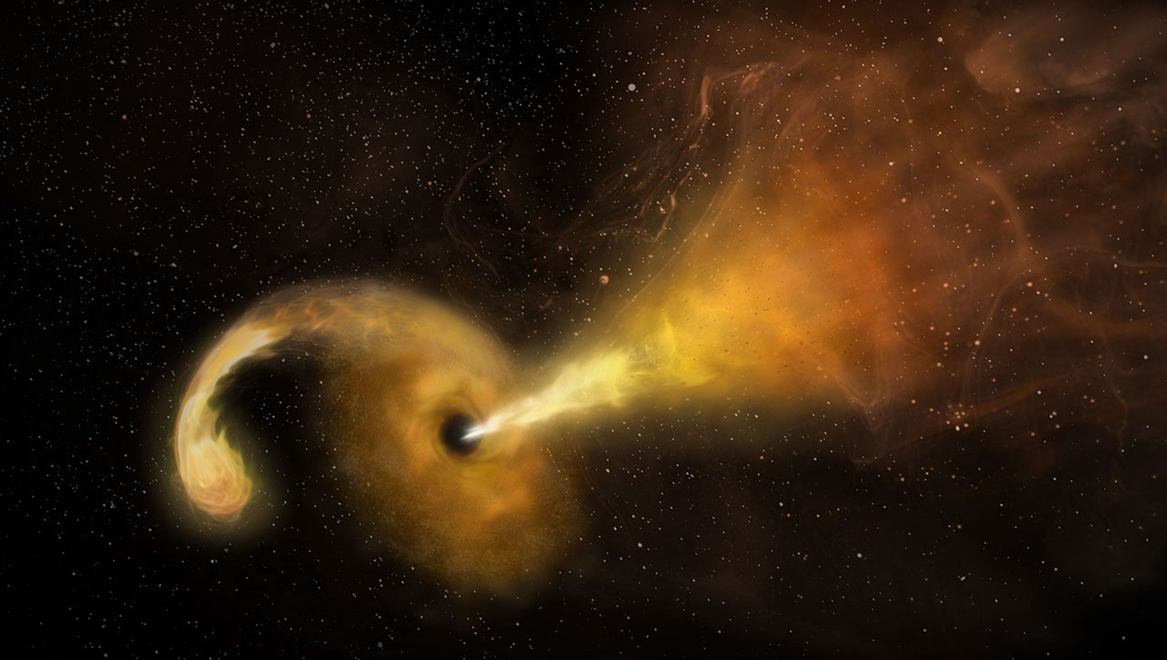
NASA’s Neil Gehrels Swift Observatory captured an “orphan” black hole lighting up as it devoured a star on the outskirts of a faraway galaxy. These phenomena are rare to begin with, and none had ever before been seen so far outside of a galaxy’s core.
“We were looking for these star-shredding events as a way to find otherwise invisible supermassive black holes wandering away from the galactic cores where they usually reside,” said Robert Stein, a research fellow at The University of Maryland, College Park and NASA’s Goddard Space Flight Center in Greenbelt, Maryland. “With this discovery, which is one of just a couple that have been confirmed so far, we’ve validated a new technique and can use it to hunt for more.”
A paper describing the results, led by Stein, was published Monday in The Astrophysical Journal Letters.
Researchers saw an ultrabright flare unleashed by a star being torn apart by extreme gravitational forces after drifting too close to a monster black hole — a phenomenon called a tidal disruption event. The black hole behind the blast weighs in at about a million times the Sun’s mass. Its existence was first flagged in November 2025 as an unusual brightening in a galaxy about 750 million light-years away by ZTF (Zwicky Transient Facility), a survey conducted by the Palomar Observatory in Southern California.
“Out of the half million flashes ZTF detects each night, our new artificial intelligence algorithm automatically recognized a flare that looked a lot like a tidal disruption event, despite its unusual location in the outskirts of a galaxy,” Stein said. For a few months, the tidal disruption event outshone its entire host galaxy in ultraviolet wavelengths, temporarily radiating with the light of about 10 billion suns.
Other telescopes, including the SOAR (Southern Astrophysical Research) telescope in Chile, followed up on the ZTF source to look at the event’s spectrum, which revealed features supporting that it was likely a tidal disruption event. Astronomers then used NASA’s Swift to look at wavelengths they can’t detect with ground-based telescopes to uncover new information. For example, Swift’s UVOT (Ultraviolet/Optical Telescope) took the blip’s temperature and found that it had quite a fever at about 54,000 degrees Fahrenheit (30,000 degrees Celsius).
“The combination of all this data helped us rule out other explanations and confidently say it’s a tidal disruption event, despite its strange location,” said Jonathan Carney, a doctoral student at the University of North Carolina at Chapel Hill, who took the first spectra that supported the flare’s interpretation as a tidal disruption event.
Hidden heavyweights
Nearly every galaxy in the universe is anchored by a supermassive black hole sitting right in the center. About once every 100,000 years, a star will drift too close to this invisible heavyweight and trigger a tidal disruption event.
While they’re rather rare in any given galaxy, scientists scour millions of galaxies for them. Each year, astronomical surveys typically spot about 30 tidal disruption events occurring somewhere in the universe.
Prior to 2024, they’d only been seen in galaxy cores. That’s partly because astronomers mainly looked for them there; after all, it’s where all the known supermassive black holes were, and you can’t get a tidal disruption event without one (the gravitational pull of lighter black holes isn’t strong enough).
Then scientists saw the telltale signs of a star being shredded 2,600 light-years from the center of its host galaxy. That inspired more astronomers to look beyond galaxy cores for similar events, and now a team has identified one more than 30,000 light-years away from a galaxy’s center.
Oddball origin story
So how did the newfound black hole become so off-kilter?
“It must have originated in a galaxy’s center, but not the one it’s in the outskirts of now,” Stein said. “We think the host galaxy’s supermassive black hole is still at its core, but the one eating the star could have started off in a small galaxy that merged with the big one we see today.”
The researchers have outlined two possibilities. Three or more galaxies may have merged together, and the gravitational tug-of-war between their central supermassive black holes may have flung the lightest black hole out to the galaxy’s edge.
Or a dwarf galaxy could be midway through a merger. As the dwarf’s stars fell into the larger galaxy, one may have passed too close to the dwarf’s supermassive black hole.
“Further discoveries could reveal the origin of this apparent ‘orphan’ black hole,” Stein said. “The key science question we want to answer is: How common are wandering black holes?”
The answer may soon be within reach. “Pointed science observations with Swift’s UVOT and XRT (X-Ray Telescope) instruments are temporarily suspended as the mission awaits an orbit boost, which is planned for this summer,” said co-author S. Bradley Cenko, Swift’s principal investigator at NASA Goddard. The spacecraft, whose primary mission ran from 2004 to 2006, is slowly sinking toward Earth due to atmospheric drag after more than 20 years of observations of the changing universe. Nudging it to a higher orbit could extend its lifetime even longer. “Once it resumes normal operations, Swift could continue searching for more examples of out-of-place black holes.”
In the coming years, scientists will use the new technique to search for disintegrating stars in observations from the newly operational Vera C. Rubin Observatory, jointly funded by the U.S. Department of Energy and National Science Foundation, in Chile and NASA’s upcoming Nancy Grace Roman Space Telescope.
“Rubin’s wide, deep surveys will reveal a much larger sample of tidal disruption events than current observatories are capable of collecting, including ones that are off-center,” Carney said. “And Roman’s space-based surveys will extend the current search zone by seeing ones that are farther away, looking back through 9 billion years of cosmic history.” Adding their observations to Swift’s and those from ground-based observatories will bring astronomers closer than ever before to completing a census of the universe’s behemoth black holes.
To learn more about the Swift mission, visit:
By Ashley Balzer
NASA’s Goddard Space Flight Center, Greenbelt, Md.
Media contact:
Claire Andreoli
NASA’s Goddard Space Flight Center, Greenbelt, Md.
301-286-1940
Share
Details
Related Terms
TechCrunch - Latest
Sam Altman is ready to decelerate
2026-07-28 20:17
Ozlo’s Sleepbuds 2 build on Bose’s sleep earbud legacy
2026-07-28 19:09
The robot NASA hired to lift a orbital telescope is tumbling out of control
2026-07-28 19:07
Waymo, robotaxi operators face fresh scrutiny over emergency response failures
2026-07-28 19:06
eBay reaches $56M settlement with e-commerce newsletter writers it terrorized in 2019
2026-07-28 18:35


